오늘 포스팅 주제는 저번 포스팅한 데이터를 이용하여 Random forest classification을 돌려보고자 합니다.
Kaggle - Breast Cancer Detection with SVM (Explanation, 설명)
본 코드는 Kaggle에서 code를 따온 다음 설명 형식으로 풀어서 공부한 것을 공유하고자 하였습니다. www.kaggle.com/mihirjhaveri/breast-cancer-detection-with-svm Breast Cancer Detection with SVM Explore an..
predictiongeek.tistory.com
1. 전처리 (preprocessing)
먼저 사용한 모듈을 한번에 import 시킵니다.
import numpy as np
import pandas as pd
import matplotlib.pyplot as plt
import seaborn as sns
from pandas.plotting import scatter_matrix
from sklearn.ensemble import RandomForestClassifier
from sklearn.model_selection import train_test_split
from sklearn.metrics import accuracy_score
from sklearn.metrics import confusion_matrix
from sklearn.model_selection import validation_curve
분석할 데이터를 저번 포스팅과 같이 세팅을 합니다.
url = "https://archive.ics.uci.edu/ml/machine-learning-databases/breast-cancer-wisconsin/breast-cancer-wisconsin.data"
names = ['id', 'clump_thickness', 'uniform_cell_size', 'uniform_cell_shape', 'marginal_adhesion', 'single_epithelial_size', 'bare_nuclei', 'bland_chromatin', 'normal_nucleoli', 'mitoses', 'class']
df = pd.read_csv(url, names=names)
df.drop(['id'],1,inplace=True)
Classification 하는 그룹 사이 어떤 관계가 있는지 확인해봅니다.
sns.pairplot(df,hue='class',markers=['o','s'],height=5)
plt.show()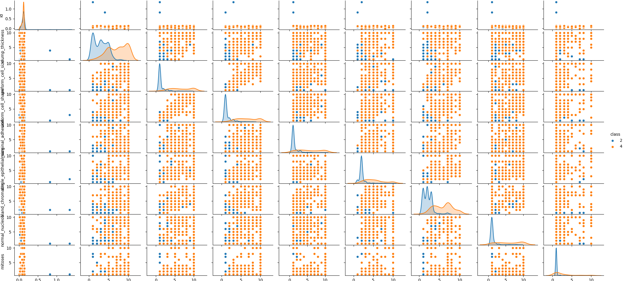
seaborn의 경우 plot사이즈 조절을 하는 방법을 잘 몰라서 확인후에 추후 포스팅에서는 이쁘게 만들도록 하겠습니다.
df.replace('?',-99999,inplace=True)
scatter_matrix(df,figsize=(18,18))
plt.show()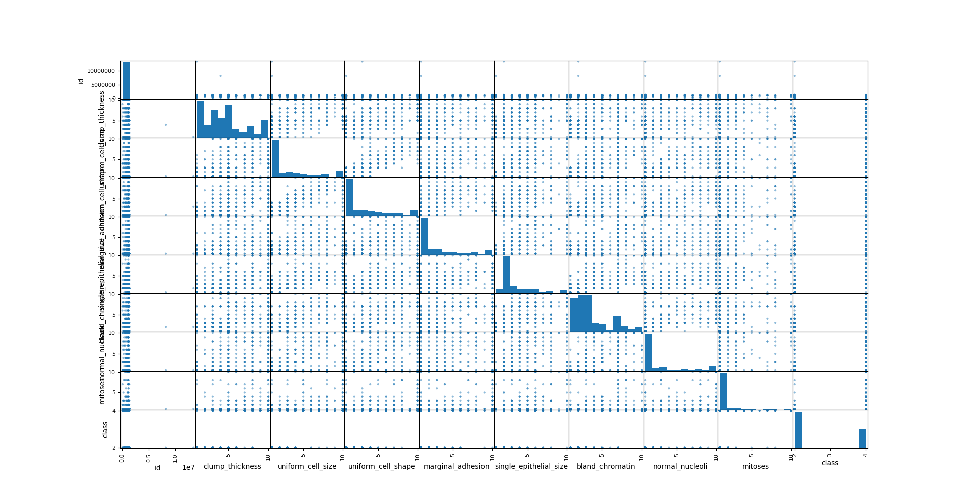
2. train set, test set 나누기
분석을 위해 train set, test set 을 나누어 줍니다.
X=np.array(df.drop(['class'],1))
y=np.array(df['class'])
X_train,X_test,y_train,y_test=train_test_split(X,y,test_size=0.25,random_state=7054)
random_state를 지정해주는 이유는 같은 결과값을 얻기 위해서 입니다.
3. model 제작과 검정
rf=RandomForestClassifier(n_estimators=100, oob_score=True,random_state=7054)
rf.fit(X_train,y_train)
### train set
train_predicted=rf.predict(X_train)
train_accuracy=accuracy_score(y_train,train_predicted)
print(f'Out-of-bad score estimate : {rf.oob_score_:.3}')
print(f'Mean accuracy score: {accuracy:.3}')

### test set
predicted=rf.predict(X_test)
accuracy=accuracy_score(y_test,predicted)
print(f'Out-of-bad score estimate : {rf.oob_score_:.3}')
print(f'Mean accuracy score: {accuracy:.3}')
결과값은 다음과 같습니다.
train set
Out-of-bad score estimate : 0.958
Mean accuracy score: 1.0
test set
Out-of-bad score estimate : 0.958
Mean accuracy score: 0.966
결과를 그림으로 확인하자면, 다음과 같습니다.
>>> cm=pd.DataFrame(confusion_matrix(y_test,predicted),columns=['2','4'],index=['2','4'])
>>> sns.heatmap(cm,annot=True)
<matplotlib.axes._subplots.AxesSubplot object at 0x7fbbb26110a0>
>>> plt.show()
>>>
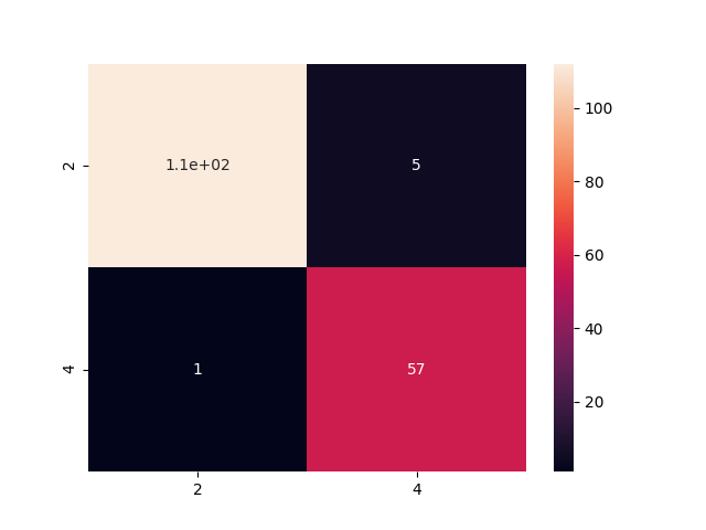
이전 포스팅한 SVM과는 다르게 2,4에 대해서 예측이 잘되나 안되나 확인한 모델이었고, 그림을 보니 잘 예측할 수 있는 것을 확인할 수가 있습니다.
SVM과 비교를 해보면 다음과 같습니다.
train set
SVM=0.9427
RF=1
test set
SVM=0.9428
RF=0.97
'python > Machine learning' 카테고리의 다른 글
| SVM 최적화 시키기 (0) | 2020.07.21 |
|---|---|
| Breast Cancer Detection with Decision tree (0) | 2020.07.17 |
| Breast Cancer Detection with K-Nearest Neighbor (KNN) (0) | 2020.07.16 |
| Breast Cancer Detection with Logistic regression (0) | 2020.07.15 |
| Kaggle - Breast Cancer Detection with SVM (Explanation, 설명) (0) | 2020.07.13 |


댓글