본 코드는 Kaggle에서 code를 따온 다음 설명 형식으로 풀어서 공부한 것을 공유하고자 하였습니다.
www.kaggle.com/mihirjhaveri/breast-cancer-detection-with-svm
Breast Cancer Detection with SVM
Explore and run machine learning code with Kaggle Notebooks | Using data from no data sources
www.kaggle.com
문제가 될시에 연락을 주시면 수정하도록 하겠습니다.
(If you have any problems, contacts me or leave a comment.)
본 코드에서 사용된 데이터는 유방암의 종류 (class, 2 for benign, 4 for malignant)를 구별하기 위하여 기타 변수들 (clump thickness (세포들의 두께?), Uniformity of Cell Size (환자안에서 세포의 크기의 일관성), Uniformity of Cell shape (세포의 모양) 등이 있음.
본 코드는 python3에서 동작을 시켰습니다.
처음 사용할 모듈들을 모두 import시켜줍니다.
(많이 해보신 분들이라면, 대략적으로 뭘 쓸지 넣을 수 있지만 대부분의 초보 혹은 중급자들은 중간중간 생각나는 데로 import를 합니다.)
>>> import numpy as np
>>> from sklearn import preprocessing
>>> from sklearn.model_selection import train_test_split
>>> from sklearn.neighbors import KNeighborsClassifier
>>> from sklearn.svm import SVC
>>> from sklearn import model_selection
>>> from sklearn.metrics import classification_report
>>> from sklearn.metrics import accuracy_score
>>> from pandas.plotting import scatter_matrix
>>> import matplotlib.pyplot as plt
>>> import pandas as pd
>>> from warnings import simplefilter
>>> simplefilter(action='ignore',category=FutureWarning)
>>> import seaborn as sns
>>>
>>> url = "https://archive.ics.uci.edu/ml/machine-learning-databases/breast-cancer-wisconsin/breast-cancer-wisconsin.data"
>>> names = ['id', 'clump_thickness', 'uniform_cell_size', 'uniform_cell_shape',
... 'marginal_adhesion', 'single_epithelial_size', 'bare_nuclei',
... 'bland_chromatin', 'normal_nucleoli', 'mitoses', 'class']
>>> df = pd.read_csv(url, names=names)
>>>특정 tsv (Tab Separated Values) , csv (Comma Separated Values)값들을 갖는 인터넷 페이지에 대해서 pandas에서 직접적으로 가져올 수가 있음.
비슷한 기능으로 pd.read_table, pd.read_excel, pd.read_sql 등이 있음.
sep를 이용하여 csv, tsv 각 종 나누는 기준을 변경할 수가 있음.
다음과 같이 바꿔서 할 수 있습니다.
>>> df = pd.read_csv(url, names=names)
>>> df_1=pd.read_table(url,sep=',',names=names)
>>> df
          id  clump_thickness  uniform_cell_size  ...  normal_nucleoli  mitoses  class
0    1000025                5                  1  ...                1        1      2
1    1002945                5                  4  ...                2        1      2
2    1015425                3                  1  ...                1        1      2
3    1016277                6                  8  ...                7        1      2
4    1017023                4                  1  ...                1        1      2
..       ...              ...                ...  ...              ...      ...    ...
694   776715                3                  1  ...                1        1      2
695   841769                2                  1  ...                1        1      2
696   888820                5                 10  ...               10        2      4
697   897471                4                  8  ...                6        1      4
698   897471                4                  8  ...                4        1      4

[699 rows x 11 columns]
>>> df_1
          id  clump_thickness  uniform_cell_size  ...  normal_nucleoli  mitoses  class
0    1000025                5                  1  ...                1        1      2
1    1002945                5                  4  ...                2        1      2
2    1015425                3                  1  ...                1        1      2
3    1016277                6                  8  ...                7        1      2
4    1017023                4                  1  ...                1        1      2
..       ...              ...                ...  ...              ...      ...    ...
694   776715                3                  1  ...                1        1      2
695   841769                2                  1  ...                1        1      2
696   888820                5                 10  ...               10        2      4
697   897471                4                  8  ...                6        1      4
698   897471                4                  8  ...                4        1      4

[699 rows x 11 columns]
>>>
>>> df.replace('?',-99999,inplace=True)
>>> print(df.axes)
[RangeIndex(start=0, stop=699, step=1), Index(['id', 'clump_thickness', 'uniform_cell_size', 'uniform_cell_shape',
'marginal_adhesion', 'single_epithelial_size', 'bare_nuclei',
'bland_chromatin', 'normal_nucleoli', 'mitoses', 'class'],
dtype='object')]
>>> df.drop(['id'],1,inplace=True)
>>>
df.replace - df 데이터 내부에 '?'를 -99999로 변경하는 function입니다.
replace(바꿀 것, 뭘로 바꿔, default=다(all))
>>> test='123,321,234,5234'
>>> test.replace(',','')
'1233212345234'
>>> test.replace(',','',1)
'123321,234,5234'
>>> test.replace(',','',2)
'123321234,5234'
>>> test.replace(',','',3)
'1233212345234'
>>>
df.drop - df에서 'id'를 제거한다. 0=row에서, 1=column에서 inplace = 본 데이터를 대체하겠다.
>>> print(df.loc[10])
clump_thickness           1
uniform_cell_size         1
uniform_cell_shape        1
marginal_adhesion         1
single_epithelial_size    1
bare_nuclei               1
bland_chromatin           3
normal_nucleoli           1
mitoses                   1
class                     2
Name: 10, dtype: object
>>> print(df.shape)
(699, 10)
>>>
loc는 label로 index되어 있는 애들에 사용함. iloc의 경우 정수로 indexing되어 있는 애들을 사용함.
df.loc[1]을 해도 위와 같이 나옴. 그냥 헤더를 보는 용도로 사용한 것 같음
>>> print(df.describe())
       clump_thickness  uniform_cell_size  uniform_cell_shape  marginal_adhesion  single_epithelial_size  bland_chromatin  normal_nucleoli     mitoses       class
count       699.000000         699.000000          699.000000         699.000000              699.000000       699.000000       699.000000  699.000000  699.000000
mean          4.417740           3.134478            3.207439           2.806867                3.216023         3.437768         2.866953    1.589413    2.689557
std           2.815741           3.051459            2.971913           2.855379                2.214300         2.438364         3.053634    1.715078    0.951273
min           1.000000           1.000000            1.000000           1.000000                1.000000         1.000000         1.000000    1.000000    2.000000
25%           2.000000           1.000000            1.000000           1.000000                2.000000         2.000000         1.000000    1.000000    2.000000
50%           4.000000           1.000000            1.000000           1.000000                2.000000         3.000000         1.000000    1.000000    2.000000
75%           6.000000           5.000000            5.000000           4.000000                4.000000         5.000000         4.000000    1.000000    4.000000
max          10.000000          10.000000           10.000000          10.000000               10.000000        10.000000        10.000000   10.000000    4.000000
>>>
Describe의 경우 R에서 Summary와 같이 기본적인 통계를 보여줌.
>>> df.hist(figsize=(10,10))
array([[<matplotlib.axes._subplots.AxesSubplot object at 0x7f1d1083cf70>,
        <matplotlib.axes._subplots.AxesSubplot object at 0x7f1d0e100550>,
        <matplotlib.axes._subplots.AxesSubplot object at 0x7f1d0e12c9a0>],
       [<matplotlib.axes._subplots.AxesSubplot object at 0x7f1d0c09e550>,
        <matplotlib.axes._subplots.AxesSubplot object at 0x7f1d0c0c89a0>,
        <matplotlib.axes._subplots.AxesSubplot object at 0x7f1d0c077d30>],
       [<matplotlib.axes._subplots.AxesSubplot object at 0x7f1d0c077e20>,
        <matplotlib.axes._subplots.AxesSubplot object at 0x7f1d0c030310>,
        <matplotlib.axes._subplots.AxesSubplot object at 0x7f1d0c007b20>]],
      dtype=object)
>>> plt.show()
>>> 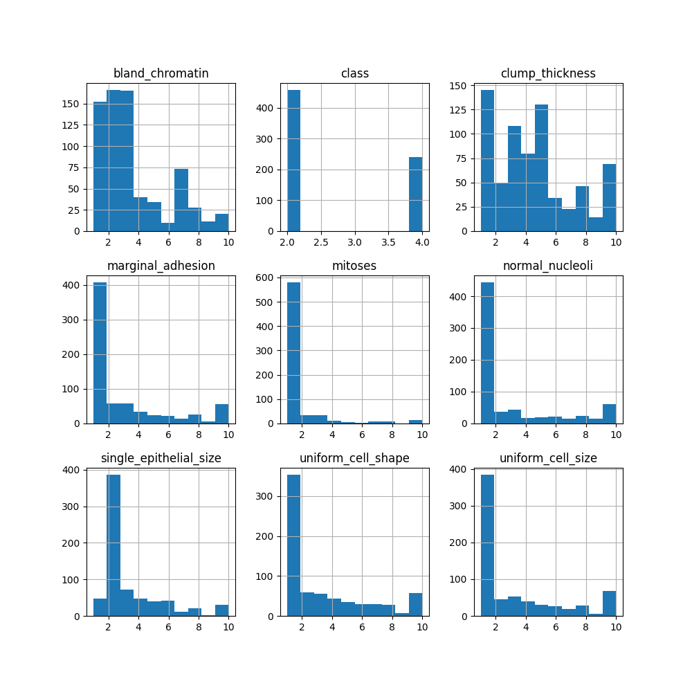
값들에 대해서 histo gram을 확인함.
>>> scatter_matrix(df,figsize=(18,18))
array([[<matplotlib.axes._subplots.AxesSubplot object at 0x7f1ca61f26d0>,
        <matplotlib.axes._subplots.AxesSubplot object at 0x7f1ca5c003d0>,
        <matplotlib.axes._subplots.AxesSubplot object at 0x7f1cd6302850>,
        <matplotlib.axes._subplots.AxesSubplot object at 0x7f1cd62b1ca0>,
        <matplotlib.axes._subplots.AxesSubplot object at 0x7f1cd626b130>,
        <matplotlib.axes._subplots.AxesSubplot object at 0x7f1cd62954c0>,
        <matplotlib.axes._subplots.AxesSubplot object at 0x7f1cd62955b0>,
        <matplotlib.axes._subplots.AxesSubplot object at 0x7f1cd6241a60>,
        <matplotlib.axes._subplots.AxesSubplot object at 0x7f1cd621fee0>],
       [<matplotlib.axes._subplots.AxesSubplot object at 0x7f1cd61d46a0>,
        <matplotlib.axes._subplots.AxesSubplot object at 0x7f1cd617ee20>,
        <matplotlib.axes._subplots.AxesSubplot object at 0x7f1cd6133610>,
        <matplotlib.axes._subplots.AxesSubplot object at 0x7f1cd615fd90>,
        <matplotlib.axes._subplots.AxesSubplot object at 0x7f1cd6113550>,
        <matplotlib.axes._subplots.AxesSubplot object at 0x7f1cd60bfcd0>,
        <matplotlib.axes._subplots.AxesSubplot object at 0x7f1cd6074490>,
        <matplotlib.axes._subplots.AxesSubplot object at 0x7f1cd609dc10>,
        <matplotlib.axes._subplots.AxesSubplot object at 0x7f1cd60543d0>],
       [<matplotlib.axes._subplots.AxesSubplot object at 0x7f1cd5ffbb50>,
        <matplotlib.axes._subplots.AxesSubplot object at 0x7f1cd5fb2310>,
        <matplotlib.axes._subplots.AxesSubplot object at 0x7f1cd5fdaa90>,
        <matplotlib.axes._subplots.AxesSubplot object at 0x7f1cd5f91250>,
        <matplotlib.axes._subplots.AxesSubplot object at 0x7f1cd5f3a9d0>,
        <matplotlib.axes._subplots.AxesSubplot object at 0x7f1cd5ef1190>,
        <matplotlib.axes._subplots.AxesSubplot object at 0x7f1cd5f1a910>,
        <matplotlib.axes._subplots.AxesSubplot object at 0x7f1cd5ec5130>,
        <matplotlib.axes._subplots.AxesSubplot object at 0x7f1cd5e79850>],
       [<matplotlib.axes._subplots.AxesSubplot object at 0x7f1cd5ea3fd0>,
        <matplotlib.axes._subplots.AxesSubplot object at 0x7f1cd5e58790>,
        <matplotlib.axes._subplots.AxesSubplot object at 0x7f1cd5e02f40>,
        <matplotlib.axes._subplots.AxesSubplot object at 0x7f1cd5dba700>,
        <matplotlib.axes._subplots.AxesSubplot object at 0x7f1cd5de4e80>,
        <matplotlib.axes._subplots.AxesSubplot object at 0x7f1ca6b115b0>,
        <matplotlib.axes._subplots.AxesSubplot object at 0x7f1ca623fd00>,
        <matplotlib.axes._subplots.AxesSubplot object at 0x7f1ca5bd1be0>,
        <matplotlib.axes._subplots.AxesSubplot object at 0x7f1cd6311700>],
       [<matplotlib.axes._subplots.AxesSubplot object at 0x7f1ca621ba00>,
        <matplotlib.axes._subplots.AxesSubplot object at 0x7f1d074e0af0>,
        <matplotlib.axes._subplots.AxesSubplot object at 0x7f1d0bfdce20>,
        <matplotlib.axes._subplots.AxesSubplot object at 0x7f1d0c023b80>,
        <matplotlib.axes._subplots.AxesSubplot object at 0x7f1d0b9166d0>,
        <matplotlib.axes._subplots.AxesSubplot object at 0x7f1d0b908a00>,
        <matplotlib.axes._subplots.AxesSubplot object at 0x7f1d0749f310>,
        <matplotlib.axes._subplots.AxesSubplot object at 0x7f1d0c0b2b20>,
        <matplotlib.axes._subplots.AxesSubplot object at 0x7f1d074a3e20>],
       [<matplotlib.axes._subplots.AxesSubplot object at 0x7f1d0b93be50>,
        <matplotlib.axes._subplots.AxesSubplot object at 0x7f1d0e12cd60>,
        <matplotlib.axes._subplots.AxesSubplot object at 0x7f1d0b995790>,
        <matplotlib.axes._subplots.AxesSubplot object at 0x7f1d0747a340>,
        <matplotlib.axes._subplots.AxesSubplot object at 0x7f1d0bfc3dc0>,
        <matplotlib.axes._subplots.AxesSubplot object at 0x7f1d0c03d940>,
        <matplotlib.axes._subplots.AxesSubplot object at 0x7f1d0e10b6d0>,
        <matplotlib.axes._subplots.AxesSubplot object at 0x7f1d078a3a60>,
        <matplotlib.axes._subplots.AxesSubplot object at 0x7f1d07851eb0>],
       [<matplotlib.axes._subplots.AxesSubplot object at 0x7f1d0780a340>,
        <matplotlib.axes._subplots.AxesSubplot object at 0x7f1d07836790>,
        <matplotlib.axes._subplots.AxesSubplot object at 0x7f1d077e1be0>,
        <matplotlib.axes._subplots.AxesSubplot object at 0x7f1d077910d0>,
        <matplotlib.axes._subplots.AxesSubplot object at 0x7f1d0774a4c0>,
        <matplotlib.axes._subplots.AxesSubplot object at 0x7f1d07776910>,
        <matplotlib.axes._subplots.AxesSubplot object at 0x7f1d07724d60>,
        <matplotlib.axes._subplots.AxesSubplot object at 0x7f1d076de1f0>,
        <matplotlib.axes._subplots.AxesSubplot object at 0x7f1d0768d130>],
       [<matplotlib.axes._subplots.AxesSubplot object at 0x7f1d076b68b0>,
        <matplotlib.axes._subplots.AxesSubplot object at 0x7f1d076610d0>,
        <matplotlib.axes._subplots.AxesSubplot object at 0x7f1d076177f0>,
        <matplotlib.axes._subplots.AxesSubplot object at 0x7f1d07640f70>,
        <matplotlib.axes._subplots.AxesSubplot object at 0x7f1d075f6730>,
        <matplotlib.axes._subplots.AxesSubplot object at 0x7f1d0759feb0>,
        <matplotlib.axes._subplots.AxesSubplot object at 0x7f1d07554670>,
        <matplotlib.axes._subplots.AxesSubplot object at 0x7f1d0757ddf0>,
        <matplotlib.axes._subplots.AxesSubplot object at 0x7f1d075345b0>],
       [<matplotlib.axes._subplots.AxesSubplot object at 0x7f1cd5d3dd30>,
        <matplotlib.axes._subplots.AxesSubplot object at 0x7f1cd5cf24f0>,
        <matplotlib.axes._subplots.AxesSubplot object at 0x7f1cd5d1bc70>,
        <matplotlib.axes._subplots.AxesSubplot object at 0x7f1cd5cd1430>,
        <matplotlib.axes._subplots.AxesSubplot object at 0x7f1cd5c7bbb0>,
        <matplotlib.axes._subplots.AxesSubplot object at 0x7f1cd5c30460>,
        <matplotlib.axes._subplots.AxesSubplot object at 0x7f1cd5c5abe0>,
        <matplotlib.axes._subplots.AxesSubplot object at 0x7f1cd5c123d0>,
        <matplotlib.axes._subplots.AxesSubplot object at 0x7f1cd5bbcb50>]],
      dtype=object)
>>> plt.show()
>>>
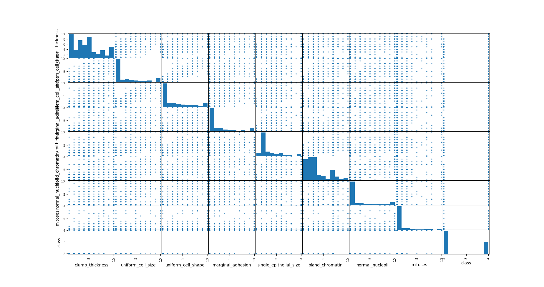
각 값들과 서로 상관성을 봄.
머신러닝에서 가장 중요한 test set, train set 나눔
>>> X=np.array(df.drop(['class'],1))
>>> y=np.array(df['class'])
>>> X_train, X_test,y_train,y_test=train_test_split(X,y,test_size=0.2)
>>>
>>> train_test_split(X,y,test_size=0.2)
[array([[4, 1, 1, ..., 3, 2, 1],
[1, 1, 1, ..., 3, 1, 1],
[1, 1, 2, ..., 2, 1, 1],
...,
[10, 3, 5, ..., 3, 10, 2],
[8, 2, 4, ..., 5, 4, 4],
[3, 2, 2, ..., 3, 2, 1]], dtype=object), array([[1, 2, 3, ..., 2, 1, 1],
[1, 1, 1, ..., 1, 1, 1],
[3, 3, 2, ..., 3, 6, 1],
...,
[4, 2, 2, ..., 2, 1, 1],
[8, 10, 10, ..., 7, 8, 1],
[7, 4, 6, ..., 4, 3, 1]], dtype=object), array([2, 2, 2, 2, 4, 2, 2, 2, 2, 4, 4, 2, 2, 4, 2, 2, 4, 4, 2, 2, 2, 2,
4, 2, 2, 2, 2, 2, 2, 2, 4, 2, 2, 4, 4, 4, 2, 2, 2, 2, 2, 4, 4, 2,
2, 2, 4, 2, 2, 2, 2, 2, 2, 2, 2, 2, 4, 4, 2, 4, 4, 2, 2, 2, 2, 2,
2, 2, 2, 4, 2, 2, 2, 2, 2, 2, 4, 4, 4, 4, 4, 2, 2, 2, 2, 2, 4, 2,
4, 4, 2, 2, 4, 2, 2, 4, 2, 4, 2, 2, 4, 2, 4, 2, 2, 2, 4, 2, 4, 2,
2, 2, 4, 2, 2, 4, 4, 2, 2, 2, 2, 4, 2, 4, 4, 4, 2, 2, 2, 2, 4, 4,
2, 2, 4, 4, 2, 4, 4, 2, 2, 2, 2, 2, 2, 2, 4, 4, 2, 2, 2, 4, 2, 2,
4, 2, 2, 2, 2, 4, 2, 2, 2, 4, 4, 4, 2, 4, 4, 2, 2, 2, 4, 2, 2, 4,
2, 2, 2, 2, 4, 2, 2, 2, 2, 2, 4, 4, 2, 4, 2, 4, 4, 4, 2, 2, 4, 2,
2, 4, 2, 4, 2, 2, 4, 2, 2, 4, 2, 2, 2, 2, 2, 4, 2, 4, 2, 2, 2, 2,
2, 4, 2, 2, 2, 2, 2, 2, 2, 2, 2, 4, 2, 2, 2, 4, 2, 4, 2, 2, 4, 4,
4, 4, 2, 2, 4, 2, 2, 2, 2, 2, 2, 2, 4, 2, 2, 4, 2, 2, 2, 2, 2, 4,
2, 4, 2, 4, 2, 2, 4, 4, 2, 2, 2, 4, 4, 4, 4, 2, 2, 4, 4, 2, 4, 2,
2, 4, 2, 4, 2, 2, 4, 2, 2, 2, 4, 4, 2, 4, 2, 2, 2, 4, 2, 2, 2, 4,
4, 2, 4, 4, 2, 2, 4, 2, 2, 4, 4, 2, 2, 2, 4, 2, 2, 2, 4, 2, 4, 2,
2, 2, 2, 2, 2, 4, 2, 2, 4, 2, 2, 2, 2, 2, 2, 2, 2, 2, 2, 4, 2, 2,
2, 4, 2, 4, 4, 2, 2, 4, 4, 2, 2, 2, 2, 2, 2, 4, 2, 4, 4, 2, 4, 2,
2, 4, 2, 4, 4, 2, 2, 2, 2, 4, 2, 2, 2, 2, 4, 2, 2, 4, 2, 2, 2, 4,
2, 2, 2, 4, 4, 2, 4, 2, 4, 4, 4, 2, 2, 2, 2, 2, 2, 4, 4, 2, 2, 4,
2, 2, 4, 2, 2, 2, 2, 4, 2, 4, 2, 2, 2, 4, 2, 4, 2, 2, 4, 4, 2, 2,
4, 2, 2, 4, 4, 2, 2, 4, 2, 4, 4, 4, 2, 4, 2, 2, 2, 2, 2, 2, 2, 2,
2, 2, 2, 2, 2, 2, 4, 4, 4, 2, 4, 2, 2, 2, 4, 4, 2, 2, 2, 4, 4, 2,
2, 4, 2, 2, 2, 2, 4, 4, 4, 2, 2, 2, 4, 2, 2, 2, 2, 2, 2, 4, 4, 4,
2, 2, 2, 2, 2, 2, 2, 4, 2, 2, 2, 2, 2, 4, 4, 2, 4, 4, 4, 2, 2, 4,
4, 4, 4, 4, 2, 2, 2, 2, 2, 4, 2, 2, 2, 2, 2, 4, 2, 4, 4, 4, 2, 2,
2, 2, 2, 2, 2, 2, 4, 4, 2]), array([2, 2, 2, 2, 4, 4, 4, 2, 2, 2, 2, 4, 4, 2, 2, 2, 2, 2, 2, 2, 2, 4,
4, 2, 2, 2, 2, 2, 2, 2, 2, 2, 4, 2, 4, 4, 4, 4, 4, 4, 2, 2, 4, 2,
4, 2, 2, 2, 4, 2, 2, 4, 2, 2, 2, 2, 2, 2, 4, 4, 4, 4, 2, 2, 2, 2,
2, 2, 4, 2, 2, 2, 2, 2, 4, 2, 2, 2, 4, 4, 2, 2, 4, 4, 2, 2, 2, 4,
4, 2, 2, 2, 4, 4, 2, 2, 4, 2, 4, 2, 2, 4, 2, 2, 2, 2, 4, 4, 2, 2,
2, 4, 2, 2, 4, 4, 4, 4, 2, 4, 2, 2, 2, 2, 4, 4, 4, 2, 4, 2, 2, 2,
4, 2, 4, 2, 2, 2, 4, 4])]
>>> train_test_split는 X,Y값 따로 받고, 알아서 비율(test_size)로 나눠서 나누어준다.
>>> seed=5
>>> scoring='accuracy'
>>> SVM_model=SVC(kernel='linear')
>>> kfold = model_selection.KFold(n_splits=10, random_state = seed)
>>> cv_results = model_selection.cross_val_score(SVM_model, X_train, y_train, cv=kfold, scoring=scoring)
>>> msg = "%s: %f (%f)" % ("SVM", cv_results.mean(), cv_results.std())
>>> print(msg)
SVM: 0.942792 (0.026192)
>>>
random selection을 위해서 seed를 먼저 선택하고, 점수의 정확도는 accuracy를 이용합니다.
KFold = n_splits만큼 돌린다는 parameter설정. random_state를 고정해주는 이유는 다른 사람도 같은 결과값을 얻기 위함.
cross_val_score = cross validation으로 KFold에서 받은 값을 이용하여 알아서 train, test 를 진행해줌. 결과는 accuracy의 평균값을 받음.
>>> SVM_model.fit(X_train,y_train)
SVC(kernel='linear')
>>> predictions=SVM_model.predict(X_test)
>>> print(accuracy_score(y_test,predictions))
0.9428571428571428
>>> print(classification_report(y_test,predictions))
              precision    recall  f1-score   support

           2       0.96      0.94      0.95        82
           4       0.92      0.95      0.93        58

    accuracy                           0.94       140
   macro avg       0.94      0.94      0.94       140
weighted avg       0.94      0.94      0.94       140

>>>
실제로 모델들을 test set에다 적용시켜서 결과 확인함.(원래는 validation set도 만드는 경우도 있음, n수가 많을 경우)
그림으로 나타내면 다음과 같습니다.
>>> cm=pd.DataFrame(confusion_matrix(y_test,predictions),columns=['2','4'],index=['2','4'])
>>> sns.heatmap(cm,annot=True)
<matplotlib.axes._subplots.AxesSubplot object at 0x7fbbaf9719a0>
>>> plt.show()
>>>
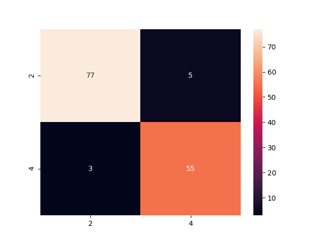
다음과 같은 결과를 확인할 수 있었습니다. 링트한 사이트와 다른 이유는 kernel을 변경해서 모델을 만들었기 때문입니다.
위의 결과는 여러분이 실습한 결과와 다를수가 있습니다. 어딘가에 random seed가 있는 것 같은데 아마 그것 때문에 결과값들이 변하는것 같습니다.
SVM에서는 Kernel이 가장 중요합니다. 이 Kernel에 대해서는 추후에 이런저런 실험을 해보도록 하겠습니다.
'python > Machine learning' 카테고리의 다른 글
| SVM 최적화 시키기 (0) | 2020.07.21 |
|---|---|
| Breast Cancer Detection with Decision tree (0) | 2020.07.17 |
| Breast Cancer Detection with K-Nearest Neighbor (KNN) (0) | 2020.07.16 |
| Breast Cancer Detection with Logistic regression (0) | 2020.07.15 |
| Breast Cancer Detection with Ramdom Forest Classification (0) | 2020.07.14 |


댓글